3D Chaotic Attractors

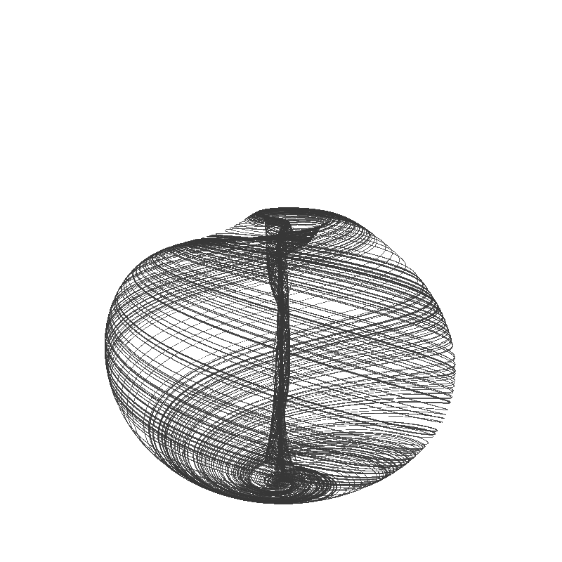
Aizawa Attractor

The Aizawa Attractor, is a spherical-shaped attractor made up from 6 parameters (a, b, c, d, e, & f). The equations generate a trajectory from an initial point (0.1, 0, 0). The equations of motion are:

$\frac{dx}{dt} = (z-b)*x - d*y$

$\frac{dy}{dt} = d*x + (z-b)*y$

$\frac{dz}{dt} = c + a*z - \frac{z^3}{3} - x^2 + f*z*x^3$

In this instance,

$a = 0.95, b = 0.7, c = 0.6, d = 3.5, e = 0.25, f = 0.1$

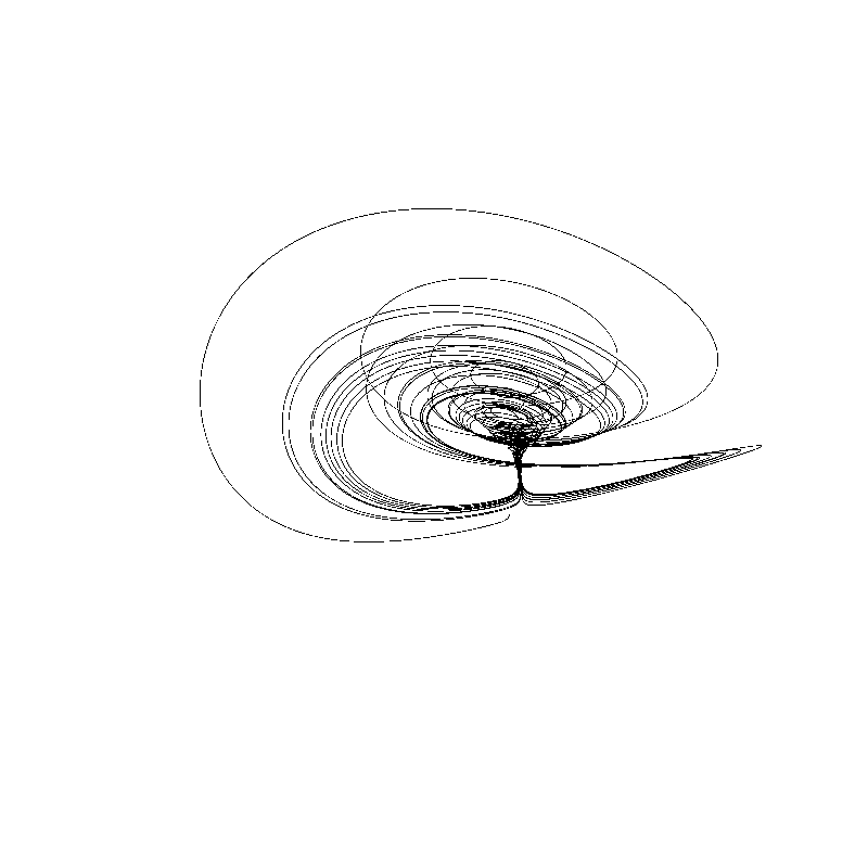
Chen-Lee Attractor

The Chen-Lee attractor is a 3 parameter system which creates a trajectory for an initial point (1, 1, 2). The equations to generate it are:

$\frac{dx}{dt} = a*x - y*z$

$\frac{dy}{dt} = b*y + x*z$

$\frac{dz}{dt} = d*z + \frac{x*y}{3}$

At the right,

$a = 5, b = -10, d = -0.38$

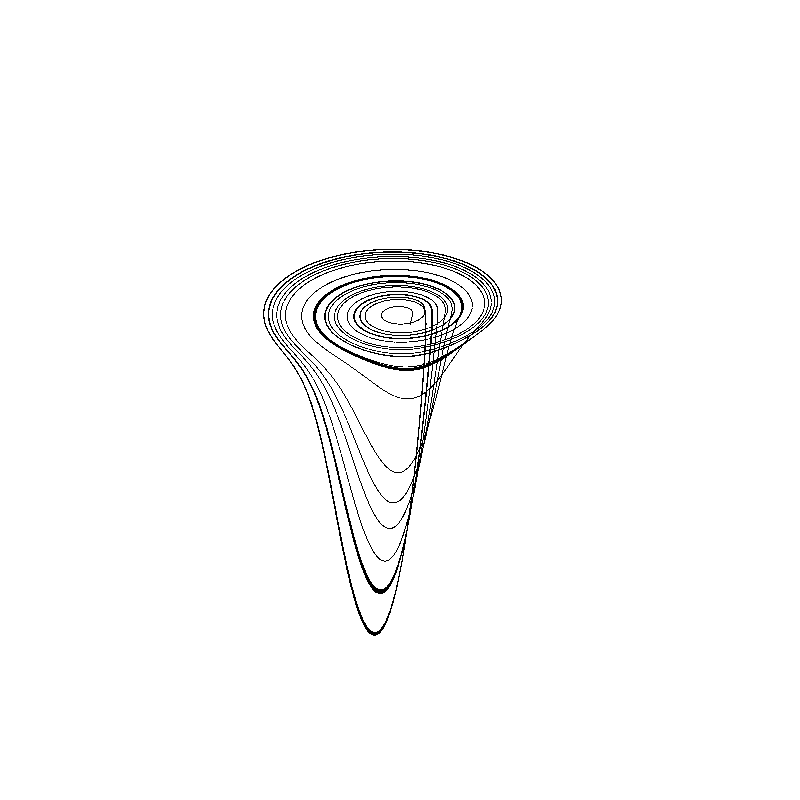
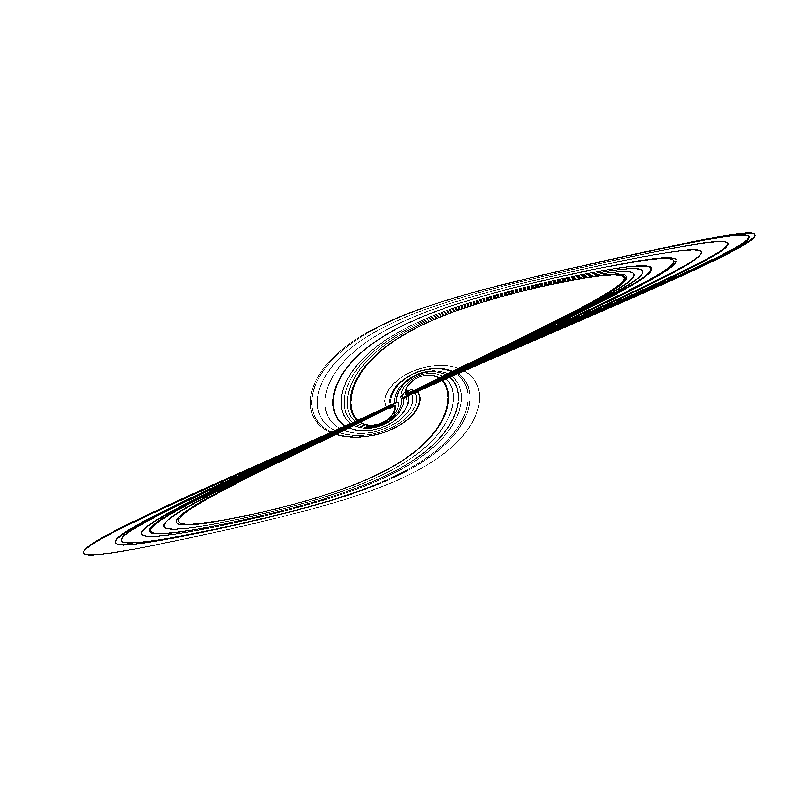
Rössler Attractor

The Rössler Attractor, created by Otto Rössler is an attractor that generates a trajectory of 3D points with 3-parameter equations. The equations are:

$\frac{dx}{dt} = -y - z$

$\frac{dy}{dt} = x + a*y$

$\frac{dz}{dt} = b + z*(x - c)$

At the left,

$a = b = 0.2, c = 5.7$

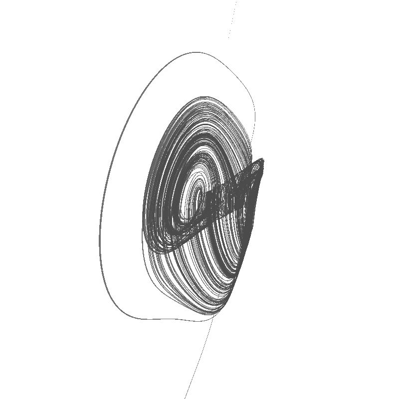
Arneodo Attractor

The Arneodo Attractor is a 3-parameter system that is generated by tracing the trajectory from an initial point. The equations to generate it are:

$\frac{dx}{dt} = y$

$\frac{dy}{dt} = z$

$\frac{dz}{dt} = -a*x - b*y - z + c*x^3$

At the right,

$x_0 = 1, y_0 = 1, z_0 = 0$

$a = -5.5, b = 3.5, d = -1$

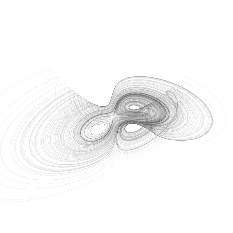
Sprott B Attractor

The Sprott B attractor was named for Clint Sprott. It has 4 parameters and is drawn by tracing the trajectory of an initial point, (0.1, 0, 0). The equations to generate it are:

$\frac{dx}{dt} = a*y*z$

$\frac{dy}{dt} = x - b*y$

$\frac{dz}{dt} = c - x*y$

At the left,

$a = 0.4, b = 1.2, c = 1$

Sprott-Linz F Attractor

The Sprott-Linz F attractor is named for Clint Sprott and Stefan Linz. It is an example of an attractor with one equilibrium for any value $a$ . It is a one-parameter system, and is generated by plotting the trajectory of an initial point (0.1, 0, 0). The equations to generate it are:

$\frac{dx}{dt} = y + z$

$\frac{dy}{dt} = -x + a*y$

$\frac{dz}{dt} = x^2 - z$

At the right,

$a = 0.5$

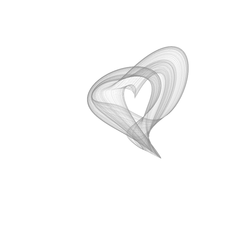
Dadras Attractor

The Dadras Attractor is a system with 5 parameters, and is created by plotting the trajectory of an initial point $(1, 1, 0)$ . The equations to generate it are:

$\frac{dx}{dt} = y - p*x + o*y*z$

$\frac{dy}{dt} = r*y - x*z + z$

$\frac{dz}{dt} = c*x*y - e*z$

At the left,

$p = 3, o = 2.7, r = 1.7, c = 2, e = 9$

Halvorsen Attractor

The Halvorsen Attractor has 1 parameter and is generated by plotting the trajectory of the points $(x, y, z)$ with initial values $(0.1, 0, 0)$ . It is generated by the equations:

$\frac{dx}{dt} = -a*x - 4*y - 4*z - y*y$

$\frac{dy}{dt} = -a*y - 4*z - 4*x - z*z$

$\frac{dz}{dt} = -a*z - 4*x - 4*y - x*x$

At the right,

$a = 1.4$

3D Quadratic Strange Attractor

Based on ideas by Clint Sprott, the 3D Quadratic Strange Attractor is a 3D phase-space of the Quadratic Strange Attractor. It is a 30-parameter system, with the equations to generate it are:

$x_{n+1} = a_0 + a_1*x_n + a_2*y_n + a_3*z_n +$
$a_4*x_n*y_n + a_5*x_n*z_n + a_6*y_n*z_n +$
$a_7*x_n^2 + a_8*y_n^2 + a_9*z_n^2$

$y_{n+1} = a_{10} + a_{11}*x_n + a_{12}*y_n + a_{13}*z_n +$
$a_{14}*x_n*y_n + a_{15}*x_n*z_n + a_{16}*y_n*z_n +$
$a_{17}*x_n^2 + a_{18}*y_n^2 + a_{19}*z_n^2$

$z_{n+1} = a_{20} + a_{21}*x_n + a_{22}*y_n + a_{23}*z_n +$
$a_{24}*x_n*y_n + a_{25}*x_n*z_n + a_{26}*y_n*z_n +$
$a_{27}*x_n^2 + a_{28}*y_n^2 + a_{29}*z_n^2$

At the left, the parameters $a_0$ to $a_{29}$ respectively are:

$-0.875,-0.173,0.307,-0.436,0.598,$
$0.003,-0.039,0.96,-0.84,0.885,$
$0.774,0.281,-0.015,0.585,0.442,$
$-0.18,-0.535,-0.151,-0.971,-0.48,$
$0.777,0.418,0.185,0.006,0.45,$
$-0.066,0.498,0.142,-0.246,-0.939$